[CS229] Lecture 6 Notes - Support Vector Machines I
-
date_range Mar. 05, 2019 - Tuesday infosortNoteslabelcs229machine learningsvm
- Introduce Support Vector Machines (SVM)
- Created on 02/27/2019
- Updated on 03/04/2019
- Updated on 03/05/2019
- 1. Margins: Intuition
- 2. Change of Notation (from logistic regression)
- 3. Function Margins / Geometric Margins
- 4. The Optimal Margin Classifier
- 5. Lagrange Duality
- Reference
Support Vector Machine (SVM) learning algorithms are among the best “off-the-shelf” supervised learning algorithm.
1. Margins: Intuition
(03/04/2019)
The intuition is to find a decision boundary that allows us to make all correct and confident (meaning far from the decision boundary) predictions on the training examples.
2. Change of Notation (from logistic regression)
- In SVM discussion, we use $y \in \{-1, 1\}$ instead of $\{0, 1\}$ to denote the class labels.
- Rather than parameterizing linear classifier with $\theta$, we use $w, b$ as parameters, and our classifier is written as:
3. Function Margins / Geometric Margins
3.1. Function Margins
Definition of the functional margin of $w,b$ w.r.t. the training example:
- where $y^{(i)} \in \{-1, 1\}$;
- if $y^{(i)}(w^Tx+b) > 0$, then our prediction on this example is correct!
Given a training set $S = \{(x^{(i)}, y^{(i)}); i = 1, \ldots, m\}$, we also define the function margin of $(w,b)$ w.r.t. $S$ as the smallest of the functional margins of the individual training examples. Denoted by $\hat{\gamma}$:
3.2. Geometric Margins
(03/04/2019)
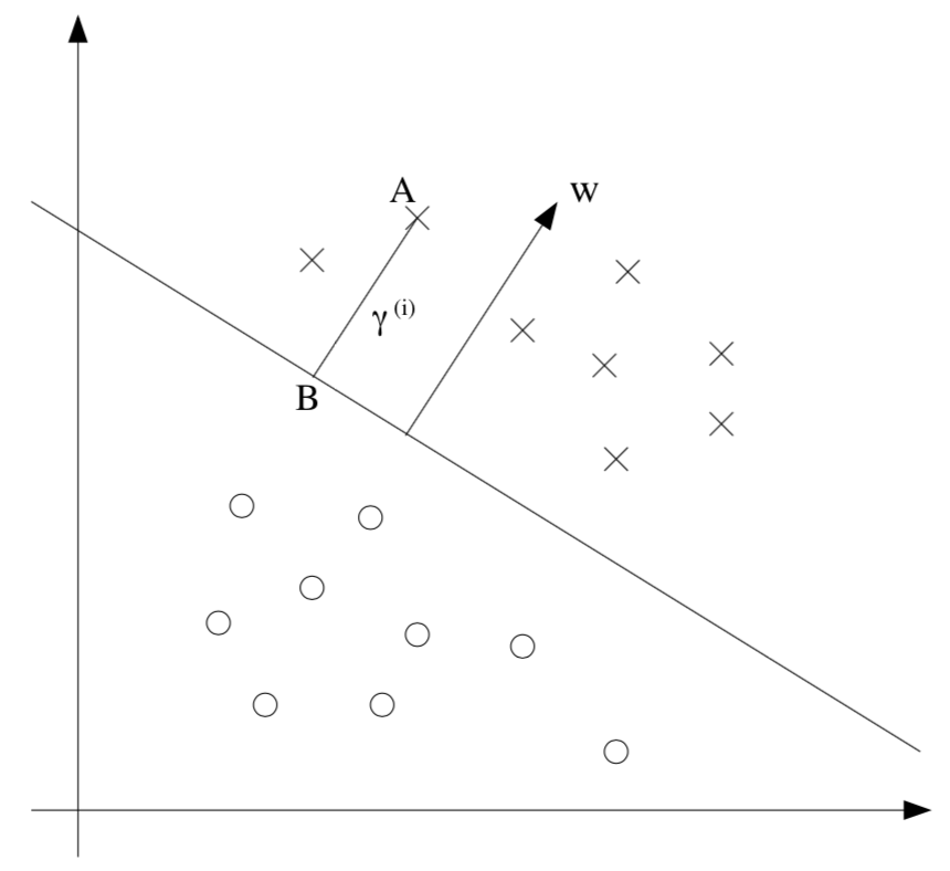
Consider the figure below:
 |
|---|
| Figure 1. Geometric Margin. |
The distance from a training sample $x^{(i)}$ to the decision boundary ($w^Tx+b=0$) is denoted as $\gamma^{(i)}$, it’s value is given by the line “AB” in Figure 1.
Derivation of geometric margins:
- Point “B” is given by $x^{(i)} - \gamma^{(i)} \cdot w / \Vert w \Vert$.
- Point “B” is on the decision boundary $w^Tx+b=0$. Hence,
- Solving for $\gamma^{(i)}$, we have:
- In order to let both “positive” and “negative” samples satisfy, we define the geometric margin of $(w,b)$ w.r.t. a training sample $(x^{(i)},y^{(i)})$ to be:
- Finally, given a training set $S = \{(x^{(i)}, y^{(i)}); i = 1, \ldots, m\}$, we also define the function margin of $(w,b)$ w.r.t. $S$ as the smallest of the geometric margins of the individual training examples:
4. The Optimal Margin Classifier
4.1. Intuition
Now, our aim is to try to find a decision boundary that maximizes the (geometric margin), since this would reflect a very confident set of predictions on the training set and a good “fit” to the training data.
Specifically, this will result in a classifier that separates the positive and the negative training examples with a “gap” (the geometric margin).
4.2. Describe the aim in math:
- Assume that we are given a training set that is linearly separable. Then, our aim is to find the hyperplane $(w,b)$ to maximize the geometric margin. The optimization problem can be written as:
- If we could solve the optimization problem, we’d be done. However, “$\Vert w\Vert=1$” constraint is nasty(non-convex), so we try to transform the problem into a nicer one:
-
This time, we’re goint to maximize $\hat\gamma/\Vert w\Vert$, subject to the functional margins all being at least $\hat\gamma$. However, this objective function $\hat\gamma/\Vert w\Vert$ is still nasty (non-convex). Therefore, we have to continue to find a better way.
-
The key idea we use here: we can add arbitrary scaling constraint on $w$ and $b$ without changing anything. Here, we introduce the scaling constraint that the functional margin of $w,b$ w.r.t. the training set must be 1:
- Plugging this into our problem above and noting that maximizing $\hat\gamma/\Vert w\Vert=1/\Vert w\Vert$ is the same thing as minimizing $\Vert w\Vert^2$, we now have the following optimization problem:
Now, the above is an optimization problem witha convex quadratic objective and only linear constraints. It’s colution gives us the optimal margin classifier.
In the following, the aim is to find a good way to solve this “constrained optimization problem”.
5. Lagrange Duality
The method of Lagrange multipliers can be used to solve constrained optimization problems (like the problems shown in the last part).
Consider a problem of the following form:
To solve this constraint optimization problems, we define the Lagrangian:
Here, the $\beta_i$’s are called the Lagrange multipliers. Then we let $\mathcal{L}$’s partial derivatives to be zero:
and solve for $w$ and $beta$, and we’d be done.
In this section, we will generalize this to constrained optimization problems in which we may have inequality as well as equality constraints.
Consider the following, the primal optimization problem:
To solve it, we start by defining the generalized Lagrangian:
Here, the $\alpha$’s and $\beta$’s arethe Lagrange multipliers. Consider the quantity:
Here, the “$\mathcal{P}$” subscript stands for “primal”. Let some $w$ be given, if $w$ voilates any of the primal constraints (i.e., if either $g_i(w) \ge 0$ or $h_i(w) \ne 0$ for some $i$), then you should be able to verify that:
Conversely if the constraints are indeed satisfied for a particular value of $w$, then $\theta_\mathcal{P}(w)=f(w)$. Hence,
Reference
shravan
